This page derives the 5-dimensional state vector used throughout the Apogee simulator.
Coordinate System Choice
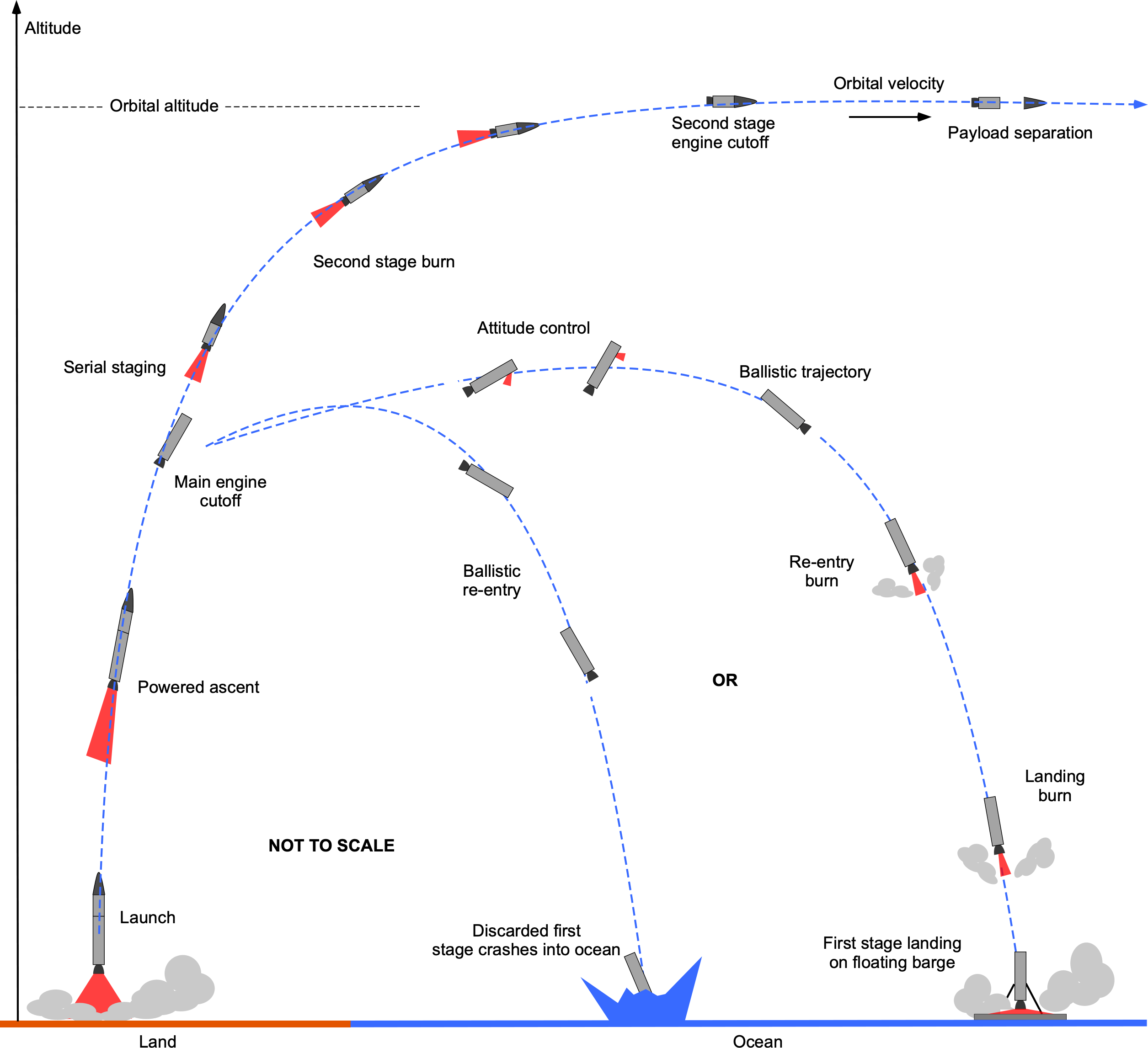
We model the rocket ascent in a 2D inertial plane centered at Earth's center. This planar approximation is valid for:
- Equatorial launches (inclination ≈ 0°)
- Short flight times (< 15 minutes)
- Negligible Earth rotation during ascent
LaTeX Reference
This section corresponds to Section 2 of nm_final_project.tex.
State Vector Definition
The complete state of the rocket at time \(t\) is described by:
State Variables
Geocentric Radius \(r(t)\)
Definition: Distance from Earth's center to the rocket.
Where: - \(R_E = 6{,}371{,}000\) m (Earth's mean radius) - \(h(t)\) = altitude above sea level [m]
Physical range: \(r \geq R_E\) (rocket is above surface)
Implementation: dynamics.py line 37
Downrange Central Angle \(\lambda(t)\)
Definition: Angular displacement measured from launch site.
Physical interpretation: - \(\lambda = 0\) at launch - At orbit insertion, typically \(\lambda \approx 0.2\) rad (≈12°)
Implementation: dynamics.py line 38
Speed Magnitude \(v(t)\)
Definition: Magnitude of the velocity vector.
Where: - \(v_r = v\sin\gamma\) (radial component) - \(v_\theta = v\cos\gamma\) (tangential component)
Physical range: - Liftoff: \(v = 0\) - Orbit insertion: \(v \approx 7800\) m/s
Implementation: dynamics.py line 39
Flight-Path Angle \(\gamma(t)\)
Definition: Angle between velocity vector and local horizontal.
Sign convention: - \(\gamma > 0\): Ascending (gaining altitude) - \(\gamma = 0\): Horizontal flight - \(\gamma < 0\): Descending
Key values: | Phase | \(\gamma\) value | |-------|---------------| | Vertical ascent | \(\pi/2\) (90°) | | After pitchover | \(\approx 80°\) | | Orbit insertion | \(\approx 0°\) |
Implementation: dynamics.py line 40
Vehicle Mass \(m(t)\)
Definition: Total instantaneous mass of the rocket.
Mass budget (Falcon 9 v1.2 FT):
| Component | Mass [kg] |
|---|---|
| Stage 1 propellant | ~411,000 |
| Stage 1 dry | 22,000 |
| Stage 2 propellant | ~107,000 |
| Stage 2 dry | 4,000 |
| Interstage | 2,000 |
| Payload | 0-10,000 |
| Total at liftoff | ~549,000 |
Implementation: dynamics.py line 41, falcon9.py
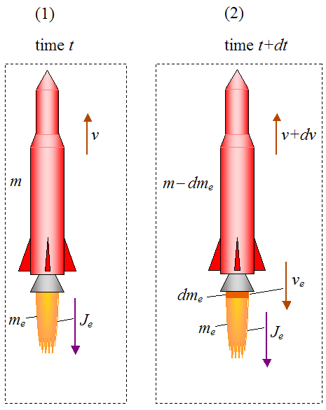
Velocity Decomposition
The velocity vector in polar coordinates:
Relating to state variables:
This decomposition leads directly to the kinematic equations derived in Equations of Motion.
Initial Conditions
For a launch from Earth's surface:
| Variable | Initial Value | Meaning |
|---|---|---|
| \(r(0)\) | \(R_E\) | On Earth's surface |
| \(\lambda(0)\) | \(0\) | At launch site |
| \(v(0)\) | \(0\) | Stationary |
| \(\gamma(0)\) | \(\pi/2\) | Vertical |
| \(m(0)\) | \(m_0\) | Gross liftoff mass |
Implementation: simulate.py lines 220-230
Why Polar Coordinates?
The polar representation offers several advantages:
- Natural gravity alignment: Gravity points radially inward (\(-\hat{e}_r\))
- Altitude is direct: \(h = r - R_E\)
- Angular momentum: \(L = r \cdot v \cos\gamma\) is simple
- Orbital insertion: Circular orbit has \(\gamma = 0\), \(v = \sqrt{\mu/r}\)
Code Implementation
@dataclass(frozen=True, slots=True)
class AscentConfig:
    earth: EarthParams
    mission: MissionParams
    vehicle: VehicleParams
    numerics: NumericsParams
The state vector indices are defined as constants:
_R = 0      # Geocentric radius index
_LAM = 1    # Downrange angle index
_V = 2      # Speed magnitude index
_GAMMA = 3  # Flight-path angle index
_M = 4      # Mass index
References
-
Battin, R.H. (1999). An Introduction to the Mathematics and Methods of Astrodynamics. AIAA Education Series. Chapter 3 - "The Two-Body Problem".
-
Curtis, H.D. (2013). Orbital Mechanics for Engineering Students. Butterworth-Heinemann. Chapter 2 - "The Two-Body Problem".
Next Steps
- Equations of Motion - Derive the governing ODEs
- Atmosphere Model - USSA76 implementation